Hamming, Blackman, and Blackman-Harris

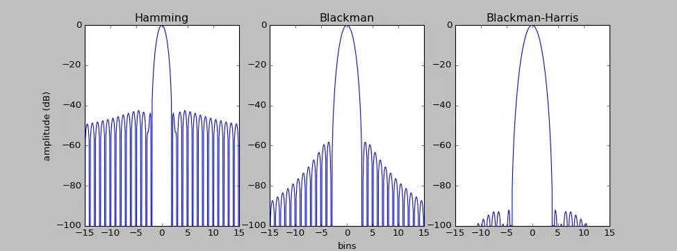
This is my implementation for some of windows used in audio applications. I chose Hamming, Blackman, and Blackman-Harris window functions. Instead of using FFT pack, I directly applied DFT since the DFT size is not too big. I scaled the amplitude for a better view. In the figure, we see their main-lobe width and side-lobes. The main lobe and the highest side lobe are important for us. I chose the small window and DFT sizes (64 and 512).

import numpy as np
import matplotlib.pyplot as plt
 
def WindowFreqResponses(M = 64, N = 512):
 
    #Window and DFT sizes have to be even
    
    #HAMMING WINDOW 	
    nh = np.arange(-M/2, M/2)
    w1 = 0.54 + 0.46 * np.cos(2 * np.pi * nh / M)   
    
    #BLACKMAN WINDOW 	
    nb = np.arange(0, M)     	       
    w2 = 0.42 - 0.5 *np.cos(2 * np.pi * nb / M) + 0.08 * np.cos(4 * np.pi * nb / M)
    
    #BLACKMAN-HARRIS 	
    nbh = np.arange(-M/2, M/2)
    w3 = np.zeros(M)
    coefficient = [0.35875, 0.48829, 0.14128, 0.01168]
 
    for i in range(0, 4):
        w3 += coefficient[i] * np.cos(2 * np.pi * i * nbh / M)
    
    w3 = w3 / M	
    
    #Taking DFT and plotting for each window 
    
    plt.subplot(131)
    DFT(w1, M, N)
    plt.title('Hamming')
    plt.ylabel('amplitude (dB)')
    plt.subplot(132)
    DFT(w2, M, N)
    plt.title('Blackman')
    plt.xlabel('bins')
    plt.subplot(133)
    DFT(w3, M, N)
    plt.title('Blackman-Harris')
    
    plt.show()
    
    return
    
def DFT(w, M, N):
    
    hWindow = int(M/2)                                    #Half of window size    		    
    fftbuffer = np.zeros(N)                               #Zero-padding
    fftbuffer[:hWindow] = w[hWindow:]
    fftbuffer[N-hWindow:] = w[:hWindow]
    
    #DFT Calculation
    
    X = np.array([])                               
                                                     	      
    for k in range(N):                              
        s = np.exp(-1j * 2 * np.pi * k * np.arange(N)/ N)
        X = np.append(X, sum(fftbuffer*s))
        
    mX = abs(X)                                           #Amplitude
    mX[mX < np.finfo(float).eps] = np.finfo(float).eps    #For machine epsilon
    mXdb = 20*np.log10(mX)                                #Amplitude in dB
    
    hDFT = int(N/2)                                       #Half of DFT size
    scaledmX = np.zeros(N)                                #For a better view
    scaledmX[:hDFT] = mXdb[hDFT:]   	
    scaledmX[hDFT:] = mXdb[:hDFT]
    plt.plot(np.arange(-N/2,N/2)/float(N)*M, scaledmX - max(scaledmX), 'b')
    plt.axis([-15, 15, -100, 0])

    return

    ###
    
WindowFreqResponses()

The results  are (approximately):

Hamming: Main lobe width is 4 bins and side-lobe level is -42.7 dB.

Blackman: Main lobe width is 6 bins and side-lobe level is -58.2 dB.

Blackman-Harris: Main lobe width is 8 bins and side-lobe level is -92 dB.

References:

[1] Mathematics of the Discrete Fourier Transform, Julius O. Smith III

[2] FFT Bin Interpolation, Ted Knowlton

[3] Windows, Matlab Documentation